No Title

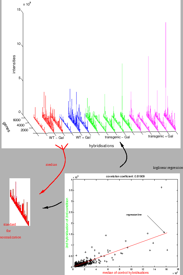
Prior to high-level analysis, data have to be normalized and filtered. In M-CHIPS, preprocessing starts with normalization of raw signal intensities. Different levels of background may result in additive offsets, or different amounts of mRNA or different label incorporation rates may lead to multiplicative distortions among the hybridizations. The normalization is based on robust affine-linear regression, i.e. it corrects for additive offsets and multiplicative distortions at the same time. The algorithms fit one measurement versus a control measurement. The performance may be judged from the scatterplot of the raw data (measurement versus control measurement, Fig. 1). In this plot, a regression line represents the multiplicative distortion (slope) and additive offset (intersect) determined by the fitting algorithm. The performance of the fit is visible in how well the regression line matches the central dense part of the cloud. Furthermore it can be observed which properties of the raw data led to an eventually suboptimal result. The scale of the plot can be switched between linear and double-logarithmic. In log scale, the regression line appears as a curve whose curvature depends on the additive offset between the two measurements.

M-CHIPS implements two algorithms as described in [1] and [2]. From amongst the options given in [1] I use the 5% quantile¹ of each hybridization as the additive offset to subtract initially. The original algorithm results in a shift of the original data to a lower intensity level, making it necessary to ignore values below a certain threshold. For correspondence analysis it is advisable to use another normalization method because low intensity signals have to be kept in order to avoid missing data. Instead, I shift all hybridizations additively to a higher range, in order to prevent overly biasing CA by the large relative error common to low intensities. This shifting is done such that the 5% quantiles coincide with that of the control measurement. For both algorithms, the set of trusted spots of unvaried expression taken into account for fitting can be specified. In most cases, the share of differentially transcribed genes is low, enabling to use the entire set for normalization. Otherwise, external control spots reporting defined mRNA concentrations or trusted housekeeping genes have to be used. For the former, defined amounts of complementary mRNA are added to the samples prior to the labelling step. For the latter, a text file is imported into M-CHIPS, listing genes that are trusted to be constitutively transcribed under the investigated experimental conditions.

In order to normalize a whole multiconditional experiment, the above algorithms are iterated. All measurements are iteratively normalized with respect to one and the same control condition, such that they can be compared afterwards. M-CHIPS discriminates between mono- and multichannel experiments, applying different control measurements and iteration steps. For monochannel (e.g. radioactive) data, each measurement is normalized versus the genewise median of the hybridizations for the control condition, resulting in absolute intensities (Fig. 1).

**Figure 1:** **Normalization of monochannel data.** Original intensity levels are shown for each hybridization and gene of a data set. It comprises four experimental conditions, each of which has been studied by three to five repetitively performed hybridizations. Necessity for normalization is stressed by apparently different intensity levels for hybridizations representing the same experimental condition. Each single hybridization is adapted to the gene-wise median of the hybridizations belonging to the control condition (red). Thus, the normalization algorithm is iterated once for each hybridization including the control hybridizations (that are adapted to their gene-wise median). The adaption is carried out by log-linear regression as shown for the third hybridization of the green condition. The scatterplot axes show arbitrary (machine dependent) intensity units.
$\resizebox*{!}{0.78\textheight}{\includegraphics{../normalization_mono.eps}}$

Filtering

Prior to high-level analysis, M-CHIPS provides a means to select genes which fulfill the following criteria: considerable absolute expression level in at least one of the conditions; substantial change relative to the control condition in at least one of the other conditions; and reproducibility in the separation from the control condition (Fig. 2) in at least one of the other conditions.

Intensity. For many arrays and experiments, the majority of genes spotted on the array are not expressed to a measurable amount. While displaying notable ratios due to measurement fluctuations, they can be eliminated by means of an intensity filter. For monochannel experiments, meaningful intensity levels are obtained by the normalization procedure. For more than one channel, apart from reflecting a low concentration of the corresponding mRNA, a low signal can be caused e.g. by high concentrations of differently labeled mRNA taking the majority of the binding sites of the spot. Therefore, multichannel intensity values are not valid as such but only in conjunction with the other channel(s) of the same hybridization. This establishes the above requirement of one and the same control condition on each hybridization for comparability. For the same reason, normalized multichannel intensities cannot be used for high-level analysis nor for intensity filtering. However, they can serve to compute ratios reflecting the relative abundance of a certain mRNA sequence under a specific condition compared to a control condition. To compute intensity levels from multichannel ratios for filtering purposes, these ratios are multiplied with an average control measurement, being the gene-wise median of the absolute intensities of the control channels. This average is a more stable basis for the determination of intensity levels. Apart from eliminating outliers by averaging repeated measurements, this procedure accounts for the above example of highly abundant differently labeled mRNA. Provided that less than 50% of the non-control conditions under study show such a high abundance of a specific mRNA, the intensity level of the control condition for that mRNA will not be low due to lack of binding sites.

Ratio. For multichannel data, ratios for each measurement are computed by dividing each normalized non-control channel gene-wise by the control channel of the same hybridization. For monochannel data, each hybridization is divided by the gene-wise median of all control hybridizations.

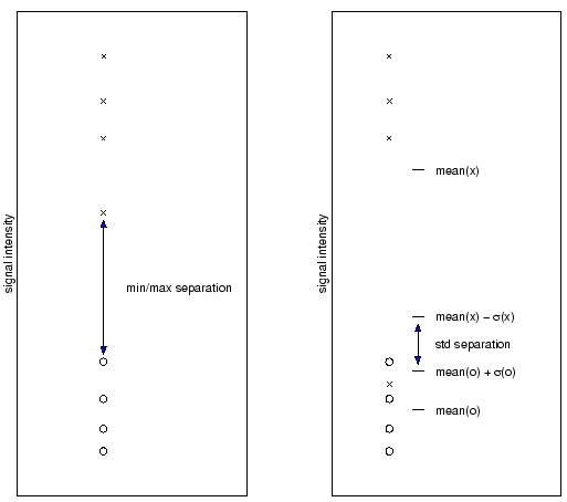
Separation. Apart from intensity and ratio filters, reproducibility measures [1] are applied to extract genes that are reproducibly up- or down-regulated. These measures integrate repeatedly performed measurements for the same experimental condition by providing the separation from a control condition (Fig. 2).

**Figure 2:** **Minmax- and standard-deviation separation.** Distributions of repeated measurements are differential among the genes, depending on the intensity level. Usually, there are not more than three to five values per gene and condition available for averaging. Here they are denoted as circles and crosses for control and non-control condition, respectively. I decided to rely on the minimal separation between two conditions (minmax-separation). Positive minmax-separation is restricted to well-sorted arrangements of the measurements of two conditions as shown in the left panel. Outliers as in the right panel lead to a negative minmax-separation. Tim Beißbarth developed the idea of diminishing the separation between the condition-means by one standard deviation ( $\sigma \protect$ ) of either condition set [1]. The standard-deviation separation is less restrictive which is preferable when higher numbers of repeatedly performed measurements are available. In these cases it is desirable to tolerate single outliers in otherwise well-sorted sets of measurements. From [1].
$\resizebox*{!}{10cm}{\includegraphics{../separations.eps}}$

Filtering. To filter out genes displaying intensities clearly above the detection limit, significant relative change and good reproducibility of this change, intensity-, ratio- and separation-thresholds can be applied. Genes not satisfying these constraints are discarded. One can also discard genes above rather than below a threshold which proved to be useful to account for saturation effects occuring e.g. if radioactively labeled arrays were exposed too long. In general, M-CHIPS provides AND-combination of three independent constraints, each of which can be defined as

Preprocessing of hybridization intensities

Normalization

Filtering

Bibliography

Footnotes